While buoyancy drives natural convection, the performance of a natural convection system can be affected by other physical phenomena and different factors such as geometry, boundary conditions, and the behavior of a fluid. Data-driven metamodels that govern real-world natural convection systems need datasets that cover the entire feature space. Moreover, some unforeseen features may become active under a different process or after a system is redesigned. Among other limiting factors, generating a new full set of simulations or experiments is time-consuming. Our methodology using transfer learning (TL) with deep neural networks (DNNs) can flexibly adapt to the expansion of the feature space when a natural convection system becomes more complicated and needs to be described more precisely.
We considered a benchmark problem in square enclosures described by the Rayleigh and Prandtl numbers. We carried out a mesh refinement study on the input space, to find the appropriate grid size to perform accurate simulations. We adopted a TL approach using DNNs to this problem and demonstrated the capability of our approach in incorporating additional input features. We built a metamodel to predict Nusselt number, Nu, as a function of Rayleigh number, Ra (the only input variable), for an air-filled enclosure. We successfully applied a DNN and transferred its learning from an air-filled enclosure to an enclosure with arbitrary fluid (i.e., Prandtl number, Pr, was added as a new input). This TL strategy is versatile and can handle straightforward metamodeling problems for many different engineering systems.
We aimed to extract a metamodel out of a physical model that numerically predicts the natural convection characteristics of a square enclosure filled with Newtonian fluid. This problem is governed by two parameters: Ra and Pr (see here for details). We consider Ra of up to 108 and Pr of greater than 0.05; however, lower Pr were also considered provided that the ratio of Ra/Pr is less than 108.
The average Nu was evaluated for different grid systems at different Pr (for the highest Ra), as summarized in Table 1. The tested grids are all uniform and structured whereas a boundary mesh is applied in which the cells adjacent to the walls were split in half to account for higher gradients near the walls. In comparison to the results obtained by an 800×800 grid system, the highest errors for the results obtained using the 200×200 and 400×400 grid systems were about 1 and 0.5 percent, respectively (for the most stringent cases). A 400×400 grid system was shown to provide precise results for Nu even for the most stringent cases. Using a single logical processor on a 2.6 GHz Intel Core i7-3720QM CPU, an average computational time of about 4,850 seconds (as high as about 13,000 seconds for low Pr) was spent on obtaining the numerical solutions using a 400×400 grid system. A 200×200 grid system (with an average simulation time of 1,300 seconds) was reliably used for Ra of up to 107 with errors of less than 0.5%.
|
Grid system |
Pr = 0.1 |
|
Pr = 1 |
|
Pr = 10 |
|
25×25 50×50 100×100 200×200 400×400 800×800 |
28.94 (14.8%) 26.78 (6.27%) 24.79 (1.65%) 25.09 (0.43%) 25.14 (0.26%) 25.20 |
|
34.65 (12.4%) 33.63 (9.12%) 31.05 (0.74%) 31.07 (0.82%) 30.93 (0.34%) 30.82 |
|
35.64 (12.1%) 35.07 (10.3%) 32.19 (1.27%) 32.13 (1.06%) 31.95 (0.51%) 31.79 |
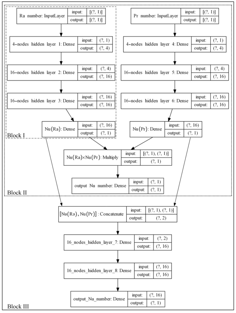
We initially generated a metamodel that predicted the variation of Nu with Ra for an air-filled enclosure (Pr=0.71). We trained an ANN as illustrated in Fig. 1 (as block I) using 30 data points (ranging from Ra=1 to 2×10⁸), without using a validation dataset during training (with the goal of lowering simulation costs). The results of testing our Ra-Nu metamodel using 10 test data points is presented in Table 2 under Step 1.

We extended our metamodel to also consider the effects of Pr. We applied the same structure as Ra (the right branch in Fig. 1) and merged the outputs of the Pr branch and block I using a Multiply layer (Keras API). We added a one-node layer after the Multiply layer to adjust for the multiplication coefficient. We froze the layers on block I, and trained the new hidden layers using data points from Step 1 as well as a new dataset of constant Ra simulation points (24 training data at a fixed Ra=105 and variable Pr ranging from Pr=10-3 to 105). We trained the ANN using 54 data points and validated it using 20 data points. We tested our ANN metamodel using a test dataset of 100 simulations using a 400×400 grid system. The test result for our ANN model is presented in Table 2 under Step 2.
|
|
Training data |
|
ANN parameters |
|
Test error |
|
Model cost |
|||||
|
Step No. |
2002 |
4002 |
|
Trainable |
Non-trainable |
|
MSE (/10-5) |
MAE (/10-3) |
RE** (%) |
|
ST (hr) |
NNT (hr) |
|
1: Block I |
23 |
7 |
|
377 |
− |
|
0.01 |
0.30 |
0.07±0.04 |
|
19.2* |
0.2 |
|
2: Block II |
42 |
32 |
|
379 |
377 |
|
22.2 |
9.35 |
2.12±2.55 |
|
42.7 |
0.8 |
|
3: Block III |
64 |
53 |
|
337 |
754 |
|
2.39 |
3.08 |
0.71±0.89 |
|
75.7 |
3.6 |
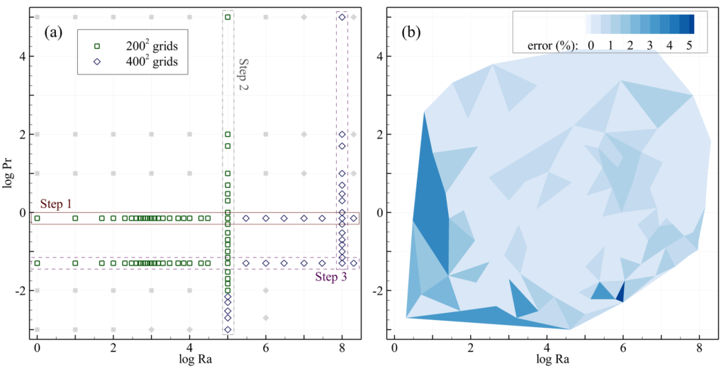
To enhance accuracy, one can remove the Multiply layer from block II and replace it with a concatenated layer followed by two additional hidden layers (Block III in Fig. 1). We froze the training on the two branches in Fig. 1 and applied the weight values from step 2 (Block II). We trained the added hidden layers in Block III using new simulation points at fixed Ra=108 or at fixed Pr=0.05 on top of the previous dataset. As presented in Table 2 (Step 3), our results on the test dataset improved remarkably after applying this procedure. The scatter graph for the different training datasets that we employed in this approach is presented in Fig. 2a. The test error contour for this approach is shown in Fig. 2b (for Step 3). Further improvements in model accuracy can be achieved after retraining the DNN from step 3 using more data. For example, using 31 additional data points (shown by grey symbols in Fig. 2a) decreased the test loss by 51% (RE = 0.45±0.66) at an increased simulation cost of 28%.
