An exhaustive metamodel using machine learning and particularly artificial neural networks (ANNs) can be used to characterize the flow and heat transfer behaviors of an engineering system. Data-driven ANN metamodels are especially useful for predicting heating or cooling processes in natural convection flows. Natural convection occurs when temperature gradients, and subsequently, density differences in a fluid induce buoyancy effects. This phenomenon has applications in various engineering systems such as nuclear reactors, heat exchangers, solar energy collectors, and electronic devices. The strength of natural convection can be quantified by the Nusselt number (Nu). Several ANN metamodels for predicting Nu in natural convection systems have been investigated using numerical simulations or by conducting experiments.
Here, we employed a transfer learning technique to predict the Nusselt number for natural convection flows in enclosures. Specifically, we considered the benchmark problem of a two-dimensional square enclosure with isolated horizontal walls and vertical walls at constant temperatures. The Rayleigh and Prandtl numbers are sufficient parameters to simulate this problem numerically. Given that the ideal grid size depends on the value of these parameters, we performed our simulations using a combination of different grid systems. This allowed us to train an artificial neural network in a cost-effective manner. By monitoring the training losses for this dataset, we were able to detect any significant anomalies that stemmed from an insufficient grid size. We then revised the grid size or added more data points to denoise the dataset and transferred the learning from our original dataset to build a computational metamodel that predicts the Nusselt number. This learning framework can be applied to other simulations that presumably have higher physical complexity while bringing the computational and training costs down.
We aimed to extract a metamodel out of a physical model that numerically predicts the natural convection characteristics of a square enclosure filled with Newtonian fluid. This problem is governed by two parameters: Ra and Pr (see here for details). We consider Ra of up to 108 and Pr of greater than 0.05; however, lower Pr were also considered provided that the ratio of Ra/Pr is less than 108. A 400×400 grid system was shown to provide precise results for Nu even for the most stringent cases. Using a single logical processor on a 2.6 GHz Intel Core i7-3720QM CPU, an average computational time of about 4,850 seconds (as high as about 13,000 seconds for low Pr) was spent on obtaining the numerical solutions using a 400×400 grid system. Nonetheless, we demonstrate that lower grid systems can provide accurate numerical solutions for limited ranges of Ra. For example, a 200×200 grid system (with an average simulation time of 1,300 seconds) can reliably be used for Ra of up to 107 with errors of less than 0.5%. Therefore, we consider a multi-grid simulation that also uses lower grid systems, wherever possible, to decrease the simulation cost in training our metamodel.
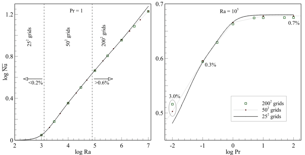
Figure 1 demonstrates Nu as a function of Ra and Pr. As can be seen in the constant-Pr curve of Fig. 1a, a 25×25 grid system reliably simulates the problem for Ra up to 103 (having a maximum difference of 0.2% relative to the results obtained from a 200×200 grid system). Likewise, a 50×50 grid system predicts Nu accurately enough provided that Ra<105 (with a maximum relative difference of below 0.6% in comparison to the result obtained using a 200×200 grid system). The validity of this statement was also assessed for different Pr, as presented in Fig. 1b for Ra=105. We conclude that we can rely on the above statement except for cases with low Pr for which coarse grid systems result in high error values (due to convergence difficulties). Therefore, we employ models having 25×25 and 50×50 simulation grids for Ra≤103 and Ra<105, respectively, and a 200×200 grid system for other cases. Nonetheless, to maintain the accuracy of the Nu result above 99%, we employ a 400×400 grid system for low Pr or high Ra. This analysis provides an approximate criterion for selecting grid sizes for different input ranges. Nonetheless, based on the errors between the original data and the ANN model, we further revised the data points by using finer grid sizes.

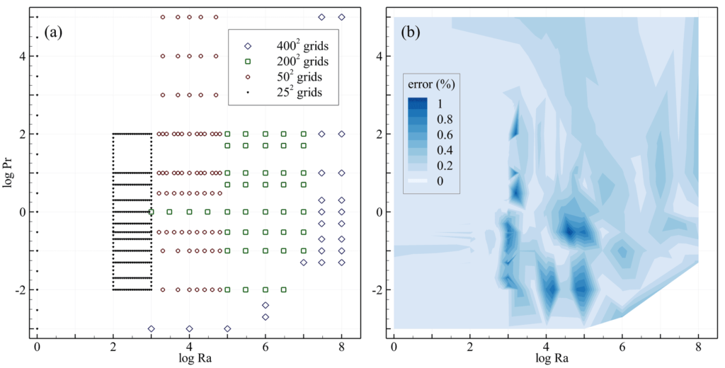
The multi-grid dataset that we used for training is shown in a scatter graph (Fig. 2a). This dataset includes a limited number of simulation data points using a 400×400 grid system (5% of the data) for cases with high Ra or low Pr. The rest of this dataset includes numerical results using 200×200 (9%), 50×50 (15%), and 25×25 grids (71%). Nonetheless, we also included simulations of higher fidelity solutions that were carried out as part of the analysis presented in Fig. 1. As can be seen in Fig. 2a, using low-cost simulations (25×25 grid systems, with an average computational time of about 40 seconds) allowed us to generate more data in the low Ra region, in order to capture the nonlinear variation of Nu for low Ra. In contrast, for higher Ra, Nu varied in a logarithmically linear manner (Fig. 1a).

An optimized ANN (as described here) was used to construct a metamodel for predicting Nu. We trained our ANN using 480 data points (in which 15% of the dataset was considered for validation during training) according to the details presented in Table 1 under “step 1”. The contour graph for the relative errors associated with the training and validation datasets used for this model is presented in Fig. 2b.
| Training data |
| Training error | Validation error |
| Model cost | ||||||
Step No. | 252 | 502 | 2002 | 4002 |
| MSE (/10-6) | MAE (/10-3) | MSE (/10-6) | MAE (/10-3) |
| ST (hr) | NNT (hr) |
1 | 340 | 73 | 43 | 24 |
| 1.12 | 0.64 | 1.77 | 0.86 |
| 53.7 | 2.0 |
2 | 339 | 68 | 65 | 36 |
| 1.03 | 0.60 | 0.93 | 0.57 |
| 79.6* | 0.8 |
* Also includes the simulation time for the data that was removed from the original dataset.
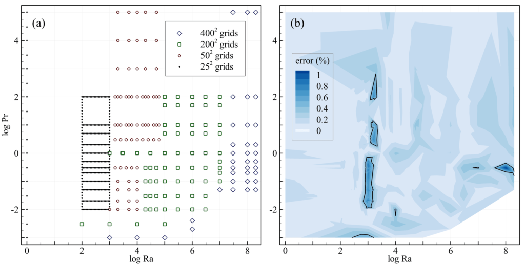
The error contour in Fig. 2b can be used to determine if the grid system for each data point was properly selected. We assumed that the source of any significant deviance in the error values in Fig. 2b was due to a lack of sufficient data points or possibly an inconsistency between the results of different grid systems. Considering these two possibilities, we revised our training dataset by adding more data points within regions with high Ra or low Pr, and replaced some of our data with higher fidelity simulation results (Fig. 3a). We fed the new dataset to our previously trained ANN to achieve an improved validation loss (by 48%) as summarized in Table 1 under “step 2”. The contour plot of the relative errors for the training and validation datasets is shown in Fig. 3b.

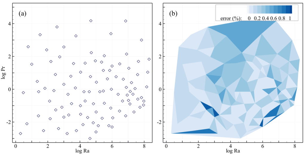
We tested our ANN metamodel using a test dataset of 100 simulations using a 400×400 grid system. Our test points were randomly drawn from normal distributions. A scatter graph for the test dataset is presented in Fig. 4a. The test result for our ANN model is summarized in Table 2. There was an improvement of 49% in the test loss (MSE) between the two steps at an added simulation cost of 46%. The test error contour for the final metamodel is presented in Fig. 4b. This metamodel predicts Nu with an error of 0.22 ± 0.21 % (the first and second terms are the mean and standard deviation of the relative errors, respectively). In Fig. 4b, the highest errors are for low Pr. As before, one can revise the training dataset based on the error contour of Fig. 3b to achieve higher accuracy.
Step No. | MSE (/10-6) | MAE (/10-3) | MRE (%) | SD (%) |
1 | 3.48 | 1.19 | 0.27 | 0.33 |
2 | 1.77 | 0.96 | 0.22 | 0.21 |
